2015-08-21
 476
476E = E 4> jeL, рвР (17.23)
ieA\di=j ieA\oi=j
E yl~dJp VseS > jsD > peP (17-24)
ieA\di=j
E tip-*?) V56S' p£P (17-25)
ieA\oi=j
E yl) -w v-v65' jeL (17-26>
PeP \ieA\ili=j J
J2xJ~n (17.27) jeL
(z,w-z;)/z;< u) v*ss (17.28)
>%eZ + VseS, ieA, peP (17.29)
*/e(0,1) VjeL (17.30)
The objective function of Eqn (17.21) aims to minimize the total average cost under all scenarios. Equation (17.22) provides the total cost under each scenario s. Equation (17.23) is the flow conservation constraint of each logistics center node. Equation (17.24) ensures that the demand should be satisfied at each demand node. Equation (17.25) ensures that the total supply of each supply node should not exceed its capacity. Equation (17.26) is the operation capacity constraint of each °§istics center node. Equation (17.27) ensures that the number of logistics centers ls restricted to a given number. Equation (17.28) ensures that the feasible solution
of model P should meet the requirement of the robust solution. Equations (17.29) and (17.30) are logical constraints of the decision variables.
17.3.3 A Min-Max Formation of RO for Road Networks [13]
Three robust improvement schemes are presented by Yin et al. [13], including sensitivity based, scenario based, and min-max for road networks under future uncertain demand. In this chapter, the improvement schemes are called robust if the resulted solutions are less sensitive to any realizations of uncertain demands (in the sensitivity-based and scenario-based schemes) or if the system performs better against the worst-case or high-consequence demand scenarios (in the min-max scheme). They formulate these different schemes as robust programs and present convenient solution algorithms. Finally, they validate their proposed models by numerical examples and simulation tests.
The min-max scheme for road networks is studied as follows.
| (17.33) |
| aeA |
| 0 — c* <d |
| c°+c+)) veV> (17-34) we VV reRH To solve this RO model, they propose a heuristic algorithm that includes an iterative procedure to obtain move directions and to generate a sequence of solutions until a convergence criterion is met. |
Consider a network G = (NA), where N is the set of nodes, and A is the set of links. Let W be the set of all origin—destination (O-D) pairs in the network. Denote travel demand between all O—D pairs as a vector q, which is assumed to be unknown but bounded by an uncertainty set Q. Rw is the set of routes between O—D pair weW, and qw is the demand between O—D pair w. 8"r= 1 if route r between O—D pair w uses link a and 0 otherwise. Denote V as the set of feasible link flow vectors (v). Denote the travel time for each link aeA as t(l(va,ca). va is the traffic flow, and ca is the capacity of link aeA. is the continuous capacity increase of link a. ha(c) is the construction cost function that is generally assumed to be nonnegative, increasing, and differentiable; В is the available budget; c"iax is the upper limit of the capacity increase; and c° is the vector of the original link capacities.
|
(17.31)
subject to

|
(17.32)
At the end of their study, they conclude some facts about the situations in which the use of each improvement scheme is preferred. Upon their conclusion, the sensitivity-based model is preferred when the fluctuations of the uncertain parameters are believed to be nonsignificant, or when the robustness approach is considered as a side improvement effort. In the other side, when it is intended to make the system performance more stable, the preferred model will be the scenario-based one. Finally, when the system performance is measured under the worst-case or high- consequence scenarios, the min-max model will be appropriate to be applied by decision makers. This model does not need any prior information about distributions of uncertain parameters.
17.4 Challenges of RO
In spite of the simplicity of implementation of this method and its applicability in modeling real-world cases, it cannot be ignored that there are several limitations in this approach. Two major shortcomings of the scenario-based RO are (1) how to determine the number of scenarios that should be included in the model to find the robust solution and (2) how to generate those scenarios and specify their related probabilities [13]. In this way, some studies have been done to overcome these limitations. For example, variance-reduction methods can be used to generate the representative scenarios.
However, we believe that the merits of developing RO would encourage the decision makers to incorporate uncertainty into the logistics networks' design phase. Besides, this field is attractive enough for further research.
References
11] D. Riopel, A. Langevin. J.F. Campbell, The network of logistics decisions, in: A. Langevin D. Riopel (Eds.), Logistics Systems: Definition and Optimization. Springer, New York, 2005.
[2] W. Klibi, A. Martel, A. Guitouni, The design of robust value-crcating supply chain networks: a critical review, Eur. J. Oper. Res. 162 (2009) 4-29.
13] N.V. Sahinidis, Optimization under uncertainty: state-of-the-art and opportunities, Comput. Chem. Eng. 28 (2004) 971 -983.
14] J.M. Mulvey, R.J. Vandcrbei, S.A. Zenios, Robust optimization of large-scale systems, Oper. Res. 43 (1995) 264-281.
15] D. Bai, T. Carpenter, J.M. Mulvey, Making a case for robust optimization models. Manage. Sci. 43 (1997) 895-907.
16] G.J. Gutierrez, P. Kouvelis, A.A. Kurawarwala, A robustness approach to uncapacitated network design problems, Eur. J. Oper. Res. 94 (1996) 362-376.
17] H. Vladimirou, S.A. Zenios, Stochastic linear programs with restricted recourse, Eur. J. Oper. Res. 101(1) (1997) 177-192.
[8] C.S. Yu, H. Li. A robust optimization model for stochastic logistic problems. Int. j Prod. Econ. 64 (2000) 385-397.
[9] V.H. Landcghcm, H. Vanmaele, Robust planning: a new paradigm for demand chain planning, J. Oper. Manage. 20 (2002) 769-783.
[10] S.C.H. Leung, Y. Wu, K.K. Lai, A robust optimization model for a cross-border logistics problem with fleet composition in an uncertain environment. Math. Comput Model. 36 (2002) 1221-1234.
[11] S.C.H. Leung, S.O. Tsang, W.L. Ng. Y. Wu, A robust optimization model for multi- site production planning in an uncertain environment, Eur. J. Opcr. Res. 181 (2007) 224-238.
[12] W. Baohua, H.E. Shiwci. Robust optimization model and algorithm for logistics center location and allocation under uncertain environment. J. Transp. Syst. Inf. Technol. 9(2) (2009) 69-74.
[13] Y. Yin, S.M. Madanat, X. Lu, Robust improvements schemes for road networks under demand uncertainty, Eur. J. Oper. Res. 198 (2009) 470-479.
[14] T. Davis, Effective supply chain management. Sloan Manage. Rev. 34 (1993) 35-46.
[15] J.M. Mulvey. A. Ruszczynski, A new scenario decomposition method for large-scale stochastic optimization. Opcr. Res. 43 (1995) 477-490.
Integration in Logistics Planning and Optimization
Behnam Fahimnia1, Reza Molaei2 and Mohammad Hassan Ebrahimi3
School of Management, Division of Business, University of South Australia, Adelaide, Australia
department of Technology Development, Iran Broadcasting Services (IRIB), Tehran, Iran
terminal Management System Department, InfoTech International Company, Tehran, Iran
18.1 Logistics Planning and Optimization Problem
A logistics system (LS) is a network of organizations, people, activities, information, and resources involved in the physical flow of products from supplier to customer. An LS may consist of three main networks or subsystems:
1. Procurement: The acquisition of raw material and parts from suppliers and their transportation to the manufacturing plants.
2. Production: The transformation of the raw materials into finished products.
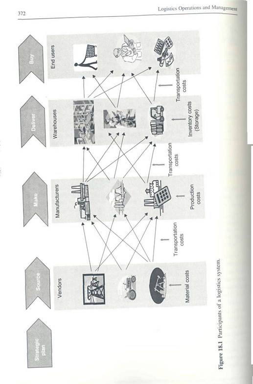
3. Distribution: The transportation of finished products from plants to a network of stocking locations (warehouses) and from there to end users.
Logistics planning (LP) is the process of integrating and utilizing suppliers, manufacturers, warehouses, and retailers so that products are produced and delivered at the right quantities and at the right time while minimizing costs and satisfying customer requirements [1]. Implementation of LS has crucial impacts on a company's financial performance and LP optimization is essential to achieve globally optimized operations. The six major cost components that form the overall logistics costs are: (1) raw material costs, (2) costs of raw material transportation from vendors to manufacturing P'ants, (3) production costs at manufacturing plants, (4) transportation costs from Plants to warehouses, (5) inventory or storage costs at warehouses, and (6) transporta- hon costs from warehouses to end users (Figure 18.1). In a logistics optimization model, the overall systemwide costs are to be minimized through effective procurement, production, distribution, and inventory management. It is widely acknowledged lhat many benefits can be achieved by treating a logistics network as a whole (integration in LS) for optimization purposes, which requires the simultaneous minimization of all systemwide costs [2].
Jftfstics Operations and Management. DOIs 10.1016/B978-0-12-385202-1.00018-9 © ini it-,

|
11 tlsevicr Inc. All rights reserved.
18.2 Significance of Integrated LP
д new approach to the analysis of LSs has been recently proposed based on the integration of decisions of different functions in production and distribution networks into a single optimization model [3]. In fact, optimization of activities in individual subsystems of LS does not guarantee the global optimization, and this has been the driving reason why researchers have changed direction toward more integrated approaches. Efficient and effective planning and control of activities within a logistics network offer opportunities in terms of cost and lead-time reductions as well as improved quality |4]. Two issues—profitability and a quicker response to market changes—can justify the call to implement effective and efficient integrated logistics optimization models.
18.2.1 Profitability
Manufacturing, distribution, and service industries have realized the magnitude of savings that can be achieved through better planning and management of complex LSs [5]. Research shows that a great portion of such financial improvements are achieved when the associated decision makings are integrated and coordinated among like-minded entities participating in the logistics network [6]. Concurrent reduction in production costs, distribution costs, and inventory holding costs can only be achieved through the effective integration of procurement, production, and distribution activities across a logistics network.
18.2.2 Quicker Response to Market Changes
Lead-time reduction is an unavoidable element of today's time-based competitions. Sajadieh et al. [7] refer to this point and cites that one important benefit of coordination in a logistics network is a more efficient management of inventories across the entire supply chain (SC) that would consequently contribute to a shorter lead time. Further, the integrated management of a logistics network can improve information flow, which would naturally lead to improved product flow and thereby shorter lead times. Many potential benefits can be obtained from lead-time reductions, including better responsiveness to market changes, more accurate forecasts, significant reductions of bullwhip effects throughout a logistics network, smaller °rder sizes, reduction in work-in-progress (WIP) inventory and inventory of finished goods, and improved customer satisfaction [8—10].
18.3 Issues in Integrated LP
^ logistics phin integrates the procurement plan, production plan, and distribution P'an. A typical integrated logistics plan aims to deal with the following problems simultaneously: (1) quantity of raw material transported from vendors to manufacturing plants; (2) quantity of each product produced at each plant during each period; (3) quantity of each product outsourced during each period; (4) Wip inventory amount stored at each plant at the end of each period; (5) inventory amount of finished products stored at stack buffers at each plant at the end of each period; (6) quantity of each product shipped from stack buffers to warehouses during each period; (7) quantity of each product shipped from warehouses to end users during each period; (8) quantity of each product shipped directly from stack buffers to end users during each period; (9) inventory amount of finished products stored at warehouses at the end of each period; and (10) quantity of each product backordered (i.e., shortage or backlogged amount for failing to satisfy the customer demand at one period) at end users at the end of each period.
An integrated logistics plan covers the planning of activities in a vast scope from raw material suppliers to manufacturers and warehouses through to end users. This large planning scope with multiple players makes the LP problem complex containing several decision variables and constraints. The problem presented by the analysis of LSs is so complex that optimal solutions are very hard to obtain [3]. The difficulties associated with this type of decision making can be further amplified by the complex maze of the network, geographical span of the SC, limited visibility, and involvement of varied entities with conflicting objectives [6]. For this reason, simplification of a real-life scenario becomes unavoidable in developing an LP model [11,12].
Most of the LP problems are classified under the category of nondeterministic polynomial-time hard (NP-hard) problems, which are very difficult to solve using ordinary planning and optimization techniques. Literature on LP and optimization indicates that past research is subject to oversimplification of real-life scenarios. Oversimplification may preclude a logistics model from functioning effectively in real- world scenarios. Hence, there is a need to extend the scope of the proposed models to perform the optimization of the detailed aggregated logistics plan. The attempt to replicate the real scenarios as closely as possible makes the LP a challenging problem [12].
Various techniques have been used to solve small- and medium-sized LP problems ranging from mathematical models, heuristics, simulation, and knowledge- based systems to the latest fuzzy programming approaches [12]. However, finding the optimal solution in a complex LP problem using the presented approaches in the literature is impossible or subject to heavy computing overheads. Consequently, there is also a need to enhance the quality and precision of the solutions for the optimization of complex real-life LP problems.
18.4 An Integrated LP Model
This section aims to formulate an LP problem consisting of multiple production plants producing different product types during several time periods and distributing the finished products from plants to various end users located in different geographical locations through a number of warehouses. Mixed-integer programming (MIP) is used for this purpose. The following subsections will discuss the key performance indicators used, assumptions, parameters and decision variables, and finally the MIP formulation of the objective function.
18ЛЛ Key Performance Indicators
The first issue in constructing a mathematical model is to determine the appropriate key performance indicator of the system. A number of performance indicators can be suggested for evaluating the performance of an LS, such as overall system costs, inventory management, delivery performance, and network responsiveness [13]. Literature on the LP models indicates that the cost-based value characteristics (e.g. total cost, profit, setup cost, delivery cost, and penalty cost) have been the most popular performance measures [12]. Cost-based optimization has a direct financial implication on system performance and clearly reflects the efficiency of the LS. The proposed model in this section is based on cost trade-off analysis, and therefore the objective functions aim to minimize the overall LS costs as the main performance measure.
18.4.2 Assumptions
There are a set of assumptions to be considered in the proposed LP model in this chapter. The procurement activities (including the raw material acquisition and its transportation to manufacturing plants) are disregarded in this model. Therefore, the proposed model is concerned with the production of multiple products in different manufacturing plants and the distribution of finished products from plants to end users (via a number of warehouses). In addition, demand is deterministic, and the aggregate demand for all types of final products in the concerned periods is assumed to be known for several periods in the near future. The aggregate demand at each end user is the total demand for each product that might have been ordered by several individuals and retailers at end users. Other assumptions include the following.
• Variety of products (/) to be produced is known.
• Number, location, and capacity of plants (m) and warehouses (vv) are known.
• Number and location of end users (e) are known.
All demands for each product have to be satisfied, sooner or later, during the planning horizon. A penalty cost will be incurred if the demand for a certain product at one period is decided to be backordcred. The backordered demands are to be satisfied in the next periods before the end of the planning horizon.
Production and distribution capacity limitations, capacity of raw material supply, and limitations in storage capacity at stack buffers and warehouses are known. To simplify the inventory management issues, a zero switch role is used in this model. This implies that the inventory levels of all products (at stack buffers and warehouses) are to be zero at the beginning and the end of the planning horizon. W1P inventory holding at manufacturing plants is disregarded in this model. Transportation costs are proportional to transportation distances. ' End users or customer zones are the locations where products are delivered to the final customers and have no holding capacity to store the products.
18.4.3 Parameters and Decision Variables
Before formulating the objective function of a model, all system inputs and decision variables must be clearly defined. Indices used for the purpose of mathematical modeling in this chapter include i for product types, m for manufacturing plants, b for stack buffers, w for warehouses, e for end users, and t for time-periods. Parameters represent the input data for a system. Therefore, a parameter is a variable with a fixed given value that is used as an input to the optimization system [12]. The following parameters are used in our model.
Die, = forecasted demand for product / at end user e in period /
Om = fixed costs of opening and operating plant m for the next planning horizon T
Ow = fixed costs of opening and operating warehouse w for the planning horizon T
Ha,/ = unit holding cost for finished product i at stack buffer b in period t
Hiw, = unit holding cost for finished product i at warehouse w in period t
HC,/„ = holding capacity (maximum units) at stack buffer b for product /' in period t
HC,V/ = holding capacity (units) at warehouse w for product i in period /
Tibwl ~ unit transportation cost for product i from stack buffer b to warehouse >v in /
Tjwe, ~ unit transportation cost for product / from warehouse w to end user e in /
Tibet ~ umt transportation cost for product i directly from stack buffer b to e in /
Pim, = unit production cost of product i at plant m in period /
OS„„, = unit outsourcing cost of product / ordered by plant m in period t
SCiel = unit backordering (shortage) cost for product / at end user e in period /
S"!;'x = maximum amount of shortage permitted (maximum backordering) for product i at
end user e in period t
Aig„,i ~ capacity hours for (he production of product i on # at plant m in t 7,,,„ = capacity units of raw material supply for product /' at plant m in period t Ец„ = the distribution capacity at stack buffer b for product i in period t Eiwl = the distribution capacity at warehouse w for product /' in period t
Decision variables are the outputs of the model or the variables in which the values need to be determined by the optimization model. The decision variables for the presented model in this chapter are listed below:
/,,,„ = quantity of product / produced at plant m in period i
ImU = quantity of product i outsourced by plant in in period /
Jihwi ~ quantity of product i shipped from buffer b to warehouse w during period t
Slwel ~ quantity of product i shipped from warehouse w to end user с during period t
Jjhel ~ quantity of product i shipped directly from stack buffer b to end user e during /
Yjh, = inventory amount of finished product /' left at buffer b at the end of period /
Ziw, = amount of product i stored at warehouse vv at the end of period /
S,v, = quantity of product i backordered at end user e at the end of period t
The integer variables include the following:
f 1, If product i is shipped from buffer b to warehouse w at period t ibw' ~ { 0, Otherwise
■ _ J 1, If product i is shipped from warehouse w to end user e at period t
nwet _ | 0, Otherwise
| { |
1, If product i is shipped from buffer b to end user e at period /
| {i |
0, Otherwise
| ( |
1, If plant m operates in period / 0, Otherwise
_., If warehouse w is open in period t
| diet - |
Gwt ~ I 0, Otherwise
| 1, If demand for product i at end user e is not satisfied at period / 0, Otherwise
18.4.4 Objective Function and Model Constraints
The objective function (i.e., cost function) in the LP problem under investigation minimizes the sum of production costs, outsourcing costs, inventory holding costs, transportation costs, and backlogging costs. The cost function for the proposed LP problem is the objective function of the model presented in Eqn (18.1). This equation consists of 10 cost components. Components 1 and 4 are the fixed costs of opening and operating plants and warehouses. These are independent of the rate and quantities of production and distribution at a plant or warehouse and may include the costs of building and facilities, amortizations of machines and tools, salaries of managers, annual insurance payments, and so on. Components 2 and 3 express production and outsourcing costs, respectively. Components 5 and 6 represent the inventory holding costs in stack buffers and warehouses, respectively. Components 7, 8, and 9 express the transportation costs for the distribution of items from plants to end users. This can be done directly from plants to end users (as in component 7) or indirectly from plants to warehouses and then from warehouses to end users (as in components 8 and 9). Component 10 stands for the shortage (penalty) costs incurred if backlogging occurs at the end users.
Min Z =
££c,,„a„ + £££/<-■** + £££L -os* +
I i m I i iii I
£ £ Gmow, + £ £ £ • у*, + E £ £ 'z<- +
H' ' i b I i w I
£ £ £ £ J>bwt ■ribwi • Fibs* + E E £ ■*+
| (18.1) |
' b и1 i i w e I
£ £ £ E fibe, ■ Tibet • F"ih, + £ £ £ • SC.V,
' bet
The proposed model is subject to capacity constraints; demand and shortage constraints; balance constraints at stack buffers, warehouses, and end users; and variables constraints.
Capacity Constraints of Plants
Raw material supply capacity restrictions:
/„„, ^ lim, v /', m, t (18.2)
Demand satisfaction constraint: The total amount of production and outsourcing for every product at all plants must meet the forecast demand for that product at the end of planning horizon (i.e., complete satisfaction of all demands for every product at the end of planning phase):
£ E С-+L) = E E ^е, v / (i8.3)
Capacity Constraints at Stack Buffers
Stack buffer capacity restriction:
Yibt — HC,/„ V i,bj (18.4)
Inventory balance at stack buffers:
| E Ji,m t + E J'bel |
| V i,b,m,t (18.5) |
Yibt ~ Yib(r-I) + \fina + I,nu] "
Capacity Constraints of Warehouses
Z,v,< HQ,., V i,w,t (18-6)
| (18.7) |
Distribution Capacity Limits at Buffers
Jibwt + E Jibe, - Eibi V t
w e
Distribution Capacity Constraint at Warehouses The distribution capacity limitation at warehouses:
V *>>' (18.8)
e
Inventory balance at warehouses:
Z,V(, - 1) + У^ Jib*, ■ Fib»! = Ji*e,' Fiwet + Z<»' V /, W, / (I 8.9)
Bocklogging Constraints at End Users Maximum allowed shortage at end users:
Siet — S(>,ax V i,e,t (18.10)
Balance equations at end users: The shipments of a product to an end user satisfy the demand for that product; otherwise some amount of shortage would appear.
Jiwel + Jibel = D'«~ ' + 5'>C " •)' - 1) V e> t (18.11)
Zero Switch Role
]£>*'= EK"»=0 V i,b (18.12)
1=0 t=T
Z<»' = Y,Zi»' = 0 V (18.13)
1 = 0 t = T
Nonnegativity Restriction for all Decision Variables
| (18.15) |
/(W> 0 V i,m,t (18.14)
C^O V i,m,t
Jibw,> о V i,b,w,t (18.16)
4*/-° v (18.17)
У(;р/>0 V i,b,e,t (18.18)
K,„,>0 V /,b,t (18.19)
Ziw, > 0 V />,/ (18.20)
5;>f>0 V (18.21)